For all you CPAs on the East Coast who are suffering through the blizzard and looking for something to do - check this out.
Free accounting game. Yes- an accounting game!
So, if you are sitting at home looking out the window at the piles and piles of snow ( or sitting in an airport!) , give this a try. Something to do. Actually it has been around for awhile and I have a link on my site to it but it's late on Friday and this is all I could come up with.
Check out http://www.revenuerecognitionchallenge.com/
a free online accounting game. Yes- that's right... free accounting game . If you report different revenue types correctly as unexpected scenarios occur and pass the "Schmarbanes-Schmoxley"audit, your stock price goes up and fireworks go off!
It's fun in a nerdy way... what I can say!
Have a good weekend and stay warm.

Software examples that you can easily understand and immediately apply to your own business needs.

Friday, February 26, 2010
Thursday, February 25, 2010
Cumulative Totals
Sometimes it is the easy stuff that escapes us.
Below is a screenshot showing how to create a cumulative total.
In the example below, I want to create a Running Total and track my T-Shirt Returns.

Why this works:
The $B$3 creates an absolute cell reference so that as the formula is copied down, it always goes back and refers to B3.
If you click in cell D4, after you create the formula, you would see that the formula has now changed to
=SUM($B$3:B4). The first cell reference is an absolute and anchors the cell reference in place but the second cell reference moves down a row.
The formula at D15 would of course read as =SUM($B$3:B15).
Below is a screenshot showing how to create a cumulative total.
In the example below, I want to create a Running Total and track my T-Shirt Returns.
- Click in cell D3 and type =SUM($B$3.B3)
- Press Enter
- Copy the formula down.

Why this works:
The $B$3 creates an absolute cell reference so that as the formula is copied down, it always goes back and refers to B3.
If you click in cell D4, after you create the formula, you would see that the formula has now changed to
=SUM($B$3:B4). The first cell reference is an absolute and anchors the cell reference in place but the second cell reference moves down a row.
The formula at D15 would of course read as =SUM($B$3:B15).
Wednesday, February 24, 2010
View Multiple Worksheets in the Same Workbook
SEE MULTIPLE WORKSHEETS IN THE SAME WORKBOOK AT ONCE
Frequently people like to look at more than one worksheet in their workbook and flipping back and forth can be bothersome.
So, if you want to view 2 or more worksheets at the same time on your computer screen all you have to do is open a second window.
Select the View Tab and then in the Window group, click New Window.
It doesn’t look like anything happens when you do this however if you look up at the title bar, you will now see a :2 after the file name to show that a second copy (window) has been made.
You can then use each window to display and edit different parts of the same workbook.
The files are mirror images of each other and any change is actually appearing in both at the same time.
Tip: Close out the :2 version first and then you will see the :1 disappear from the original. If you close out the :1 first, it is not a big deal, however you will always have that :2 after the name and then you are always wondering whatever happened to Version 1. :)
Tuesday, February 23, 2010
Smart Tables in Excel 2007
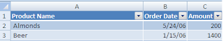
Excel 2007 offers a wonderful feature that not many people are aware of. It is called a Smart Table and, in my mind, is basically an advanced version of Excel 2003’s List feature.
Excel considers a list or table to consist of data that is adjacent and does not contain a totally empty column or a totally empty row.
With the Table feature, you can have new data formatted as you enter it, shade alternate rows, instantly sum up the right column and quickly name the table.
The most exciting feature however is that tables are dynamic. As you add or delete data, Excel automatically updates and formats the table. So, what does this really mean for you? It means that if you base a chart, a pivot table or a formula on a table, as data changes in the table, it will automatically update the chart or whatever it is based on. This ensures that you are working with the most current data.
CREATE A TABLE
To create an Excel table

The table feature automatically bands and shades every second row and it applies filter arrows to the column headings. A definite timesaver.
When the table is created, a contextual toolbar also appears.
It allows you, among other things, to quickly sum a column, name the table, change formatting styles as well as remove duplicates.
 Adding data into the spreadsheet is not any different than what you have done before – you simply select a cell in the row immediately below the last row and type the value in.
-If you enter a formula in the adjacent column, Excel will automatically copy it down the entire table and format it.
-If you enter data in the adjacent row, Excel will automatically format it so that it matches the table.
To me, the exciting part of the table is that when you add the total row, Excel automatically calculates the values in the rightmost column. You can change that summary operation or add a total to another column easily.
To Create a Total Row
-Make sure your cursor is in the table
-Click on the Design tab under the new Table Tools tab
-Click Total Row

The last row of your total now displays the sum of the right most column.

Excel considers a list or table to consist of data that is adjacent and does not contain a totally empty column or a totally empty row.
With the Table feature, you can have new data formatted as you enter it, shade alternate rows, instantly sum up the right column and quickly name the table.
The most exciting feature however is that tables are dynamic. As you add or delete data, Excel automatically updates and formats the table. So, what does this really mean for you? It means that if you base a chart, a pivot table or a formula on a table, as data changes in the table, it will automatically update the chart or whatever it is based on. This ensures that you are working with the most current data.
CREATE A TABLE
To create an Excel table
- Type your data into the worksheet as you normally would
- Make sure that you include column headings
- Do not leave any empty rows or columns
- Click in the data and press CTRL+T.

- Click OK.
The table feature automatically bands and shades every second row and it applies filter arrows to the column headings. A definite timesaver.

When the table is created, a contextual toolbar also appears.
It allows you, among other things, to quickly sum a column, name the table, change formatting styles as well as remove duplicates.

-If you enter a formula in the adjacent column, Excel will automatically copy it down the entire table and format it.
-If you enter data in the adjacent row, Excel will automatically format it so that it matches the table.
To me, the exciting part of the table is that when you add the total row, Excel automatically calculates the values in the rightmost column. You can change that summary operation or add a total to another column easily.
To Create a Total Row
-Make sure your cursor is in the table
-Click on the Design tab under the new Table Tools tab
-Click Total Row

The last row of your total now displays the sum of the right most column.

Monday, February 22, 2010
Creating and Using a Template
Templates
Templates are a useful tool that are often forgotten or overlooked. People use them in Word to create invoices and other standardized forms but never think to apply that standardization to their Excel workbooks.


- If you use custom formats or find yourself applying a standardized formatting to every Excel document that you create (be it fonts, column widths, number formats )then you should consider creating a template.
- It can also be useful if you are working with others on a project such as a budget and want to ensure that the setup and formatting are all the same. You can create a template and then distribute it.
- Create a worksheet and set it up as you want
- Go to the Office Button
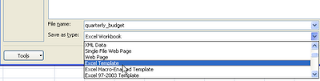
- Select Save As
- Click on the drop-down arrow beside Save As Type
- Select Excel Template or Macro-Enabled Template if your workbook contains macros
 Enter a name for the template
- Click Save

The default is that the template is saved inside the Template Folder. However, you can save it elsewhere.
============================================
If you have saved it in the default Template folder, it is extremely easy to retrieve.
Simply click on the Office ButtonSelect New
Select My templates... from the left column
Select My templates... from the left column

Select the template you want and click OK

Since you saved the file as a Template, after you complete work on it and go to save it, Excel will prompt you to name it something else so that the template is not overwritten.
Friday, February 19, 2010
Fixed Decimal Places
Macro Tip for Fixed Decimal
I have this Fixed Decimal Place tip, which is below, in my Must Know Excel Tips Tricks and Tools for the CPA.Ebook. Eric Robinson read my tip and sent me his own. He shared a macro he uses to switch back and forth between no decimal place and decimal places. Switching back and forth can be tedious if you are, for example, entering check numbers (no decimal) and check amounts (2 decimal places). I have added it below. Thanks so much Eric.
Sub ToggleAutoDecimal()
'
' ToggleAutoDecimal Macro
' Macro recorded by Eric Robinson to handle fixed decimal places
'
Application.FixedDecimal
= Not (Application.FixedDecimal)
End Sub
Fixed Decimal Place
I was teaching an Excel class a few years back and briefly mentioned the Fixed Decimal Place feature. My goodness, half the class was enthralled with it. It seemed to be the biggest thing they had seen since sliced bread! (Hmm. I guess I need to come up with a more up to date expression particularly since I buy unsliced bread.)If you are a numbers person then you too may appreciate this feature. If you need to enter columns of numbers, with a fixed number of decimals, into a worksheet then make your job a lot easier by having Excel enter the decimals for you. For example, I set the fixed decimal feature to 2 and then in Cell B2, I typed 1234 and Excel displays it as 12.34. It can be a bit of a time saver.

When you turn the feature on, the default is 2 decimal places but you can change it to whatever you want.
=======================================================================
If you are constantly dealing with large numbers and would like them to be truncated to the same decimal place then you can also use this feature.

In the example to the left, I typed original values in Column A, I then turned on the fixed decimal place feature to 2 decimal places and when I typed in the same numbers, Excel changed them.
So, when I typed 500000 into cell B2, Excel changed it to 5000. In Column C, I changed the fixed decimal place feature to 3 and when I typed in 500,000, it changed it to 500.
You get the idea. So, this may really excite you and you may find it useful however please be aware that Excel now considers cell C2 to be 500. If I add C2 + 0, the answer I get is 500 not 500,000 even if you have turned the fixed decimal place feature off.
If you don't want every number in your spreadsheet truncated then you need to type the decimal place in yourself.
For example, if the fixed decimal feature is on and set to 2 decimal places, if I type 200.00 in a cell, Excel will change it to 200 however if I type 200 into a cell, Excel will display it as 2.

Here are the steps in case you want to look at it
Excel 2003
- Select the Tools menu.
- Select Options.
- Select the Edit tab.
- Select the Fixed decimal Places checkbox.
- Select the appropriate number of places.
- Click OK.
Other Versions:
- Click File (Excel 2010-2016) or Office Button (Excel 2007).
- Select Options (at the very bottom of the dialog box).
- Click on Advanced.

- Put a checkmark in Automatically insert a decimal point and select the number of Places.
- Click OK..
Have a great day!
Thursday, February 18, 2010
Deleting Blanks
Often when you import data, you end up with a lot of BLANK ROWS.
Here is an easy way to get rid of them.
Excel 2003 method:
Excel 2007 method:
You could also right-click and select Delete instead of going to the Ribbon if you preferred.
Here is an easy way to get rid of them.
Excel 2003 method:
- Select your data
- Select Edit and Go To
- Click Special…
- Click OK
- Select Edit
- Select Delete...
- Select Entire Row
- Click OK
Excel 2007 method:
- Select your data
- Select Find and Select on the Home Tab
- Select Go To Special..
- Select Blanks
- Click OK
- Select the drop-down arrow under Delete in the Cells group on the Home Tab
- Select Delete Entire Row
- Click OK
You could also right-click and select Delete instead of going to the Ribbon if you preferred.
Tuesday, February 16, 2010
More Duplicates
I realized that Method 3 only showed you how to identify numbers. If you have a mix of numbers and text, you may find this example more useful.

I would be glad to share it here.

In this example, I had values in Column A and Column B and I wanted to identify which were duplicates.
I typed the following formula =IF(ISERROR(MATCH(A1,$B$1:$B$5,0))," ",A1) in Column D and then copied it down. This formula tells Excel to Compare Column A against Column B and to identify any values that match. Excel found that there was a match for may in Column B and there was a match for the value 2 in Column B so those are the only values that display in Column D.
If you do anything else with duplicates, let me know.
I would be glad to share it here.
Tuesday, February 9, 2010
Duplicates- Conditional Formatting
Duplicates
In Excel 2007, it is easy to remove duplicates.
You select your data, and then select Conditional Formatting on the Home Tab.
Select Highlight Cell Rules and then select Duplicates.
A dialog box comes up for you to select a fill/highlight color for the duplicates.


In Excel 2007, it is easy to remove duplicates.
- Select your data
- Click on the Data tab
- Click Remove Duplicates
Easy..Peasy.. but sometimes you might actually want to look at what Excel is removing but Excel only tells you how many duplicates were removed - it doesn't show them to you.
You can easily identify duplicates and/or unique values using Excel 2007's Conditional Formatting.
Using the basics of conditional formatting merely formats the duplicate cells. In this case, it formats both the original and any other instances of it.
Select Highlight Cell Rules and then select Duplicates.
A dialog box comes up for you to select a fill/highlight color for the duplicates.

An alternative method:
You can also select New Rule and then select Format only unique or duplicate values which is an alternative way to get to the same place.

There is actually a lot of 'stuff" on duplicates as it is a problem everyone faces so perhaps I will continue this conversation tomorrow.
Monday, February 8, 2010
Duplicates
Great game although The WHO vocals and the ads were a bit of a disappointment.
DUPLICATE VALUES
I've had a number of emails and conversations lately about identifying duplicate values.
Using Conditional Formatting in Excel 2007 makes it relatively easy but not everyone has Excel 2007.
Let's start with Excel 2003:
Let's say that you have a column of numbers in B4:B16 and you want to identify duplicates.
Method 1:
Sort - Easy but sometimes you can't or don't want to manipulate your data.
Method 2: Click in cell C4 and type


You will have a column of TRUE and FALSE. You can manually delete them or highlight them. The problem with this method is that Excel labels both numbers are TRUE - there is no differentiation between the original and the duplicate.
To get around this, try =IF(ISNUMBER(MATCH(B4,$B$3:B$3,0)),"Duplicate","Unique").
This will label the original as Unique but any other instances will be labeled as a Duplicate.

Method 4: This method is actually available in Excel 2003 and Excel 2007.
You can use the Advanced Filter function under the Data menu or tab and select Unique Only.
To be honest, I have mixed results with this so double-check your answer.
Select the column of numbers and then go to the Data tab or menu and select Advanced Filter.
Click copy to another location
Enter a cell to Copy To:
Put a checkmark in Unique Records Only
Click OK.

Well, it's getting late. Tomorrow I'll talk about how to identify Duplicates in Excel 2007.
Friday, February 5, 2010
It's Friday!
Sorry.. I got behind and just realized that it is 6pm.
I am looking out the window at about 5 inches of snow. An absolutely beautiful sight.
Stay warm.
Watch those great Superbowl Ads and cheer for your preferred team.
Have a great weekend.
Patricia
Patricia


Thursday, February 4, 2010
Calculating Age or Years of service
When you are calculating age or years of service, you can't just subtract the date from the current date. You will not get the correct answer if you do that. Instead, you need to use =yearfrac() which will give you a fraction based on the number of days between the Start Date and the End Date.
The syntax is =yearfrac(today(),A1,1))
My brother's birthday is next week so let's see how old he actually is:
 38.97 sounds better than 39 doesn't it? Now, if you wanted it as a whole number you could simply use the INT() function with it.
=INT((YEARFRAC(TODAY(),A1,1)))
DATEDIF() is not documented in Excel and has to be typed in manually.
Rumor has it that it was a very popular Lotus function and back when people were transitioning there was a huge outcry over its loss and Microsoft added it in - grudgingly..ergo.. no documentation.
DATEDIF() allows you to display the date in terms of years, months or days.
The syntax is DATEDIF(start date, end date, time interval)
Time intervals include:
"Y" The number of complete years
"M" The number of complete months
"D" The number of days.
"MD" The difference between the days in start_date and end_date.
The months & years of the dates are ignored.

=DATEDIF(A1,NOW(),"Y")&" years" &" "&DATEDIF(A1,NOW(),"ym") &" months "
and the resulting answer would display as 38 years 11 months
Remember, the & joins items together and you need quotes around text. I left a space before and after the word years and months so that everything would not run together. If you don't press your space bar to get the spaces, your answer will look like this: 38years11months instead of 38 years 11 months.
When you are calculating age or years of service, you can't just subtract the date from the current date. You will not get the correct answer if you do that. Instead, you need to use =yearfrac() which will give you a fraction based on the number of days between the Start Date and the End Date.
The syntax is =yearfrac(today(),A1,1))
My brother's birthday is next week so let's see how old he actually is:

=INT((YEARFRAC(TODAY(),A1,1)))
Now- be careful - if you use the INT, his age would display as 38. After all, he is not 39 yet. Don't rush him. Just wait until next year. Egad. my baby brother is getting old.
========================================================
For those of you who remember Lotus, you can also use DATEDIF(). This function provides you with a little more flexibility. ========================================================
DATEDIF() is not documented in Excel and has to be typed in manually.
Rumor has it that it was a very popular Lotus function and back when people were transitioning there was a huge outcry over its loss and Microsoft added it in - grudgingly..ergo.. no documentation.
DATEDIF() allows you to display the date in terms of years, months or days.
The syntax is DATEDIF(start date, end date, time interval)
Time intervals include:
"Y" The number of complete years
"M" The number of complete months
"D" The number of days.
"MD" The difference between the days in start_date and end_date.
The months & years of the dates are ignored.
"YM" The difference between the months in start_date and end_date.
The days & years of the dates are ignored.
"YD" The difference between the days of start_date and end_date. The years of the dates are ignored.

If you are really into it, you can join these functions all together using & and quotes
and get something like this:=DATEDIF(A1,NOW(),"Y")&" years" &" "&DATEDIF(A1,NOW(),"ym") &" months "
and the resulting answer would display as 38 years 11 months
Remember, the & joins items together and you need quotes around text. I left a space before and after the word years and months so that everything would not run together. If you don't press your space bar to get the spaces, your answer will look like this: 38years11months instead of 38 years 11 months.
Tuesday, February 2, 2010
WEEKNUM()
One Date Function that some of you may find useful is =WEEKNUM()
This function returns the week number in the year.
If you want to find out what the current week number is you use the =TODAY() or =NOW() with WEEKNUM.
So, in the example below, =WEEKNUM(TODAY()) returned the value of 6 because today is February 2 2010.
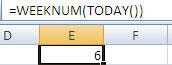
Warning: Microsoft points out that the WEEKNUM function is based on the American standard where January 1 is considered the first week of the year even though this year the first week of 2010 only had two days in it. The European standard differs as the first week of the new year has to have at least 4 days in it so this function should not be used if you are presenting or using the data where European standards are used.
Monday, February 1, 2010
I could have sworn I had blogged about Date Functions awhile ago but apparently not.
Let me start with some basics.
A lot of people struggle with Date Functions and I think a lot of the problem arises because of formatting problems as as the fact that many of the answers are volatile.
If you don't know about =TODAY() or =NOW(), you should check them out. I use them constantly.
=TODAY() returns today's date. It is a volatile function. By volatile, I mean that it changes.
Coming from Lotus - oh so long ago- I hated these functions. I think I spent 2 hours once trying to figure out what I was doing wrong - only to realize that yes you really do need the empty parentheses to get the function to work!
If I type =TODAY() in an Excel spreadsheet today, which is February 1, it will display February 1. But, if I save the spreadsheet and open it February 2, it will display February 2 without me having to do anything. Open it on March 15th and it will display March 15th.
=NOW() works the same way, only it displays the current date and the current time.
People tend to be a little wary of these because sometimes the display looks hinky..(is that word?)
=TODAY() only displays the date so if you format it as date and time, it always displays 12:00 which of course looks strange.
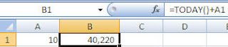
Sometimes, if you are using these functions in a mathematical calculation, Excel tries to help you out and just confuses you. For example, if I type =TODAY() + A1 and A1 contains the value 10, I expect the answer to be February 11, 2010 since 10 days from today, February 1, would be February 11th. However, sometimes Excel surprises you and gives you an answer like the one below:
Let me start with some basics.
A lot of people struggle with Date Functions and I think a lot of the problem arises because of formatting problems as as the fact that many of the answers are volatile.
If you don't know about =TODAY() or =NOW(), you should check them out. I use them constantly.
=TODAY() returns today's date. It is a volatile function. By volatile, I mean that it changes.
Coming from Lotus - oh so long ago- I hated these functions. I think I spent 2 hours once trying to figure out what I was doing wrong - only to realize that yes you really do need the empty parentheses to get the function to work!
If I type =TODAY() in an Excel spreadsheet today, which is February 1, it will display February 1. But, if I save the spreadsheet and open it February 2, it will display February 2 without me having to do anything. Open it on March 15th and it will display March 15th.
=NOW() works the same way, only it displays the current date and the current time.
People tend to be a little wary of these because sometimes the display looks hinky..(is that word?)
=TODAY() only displays the date so if you format it as date and time, it always displays 12:00 which of course looks strange.
Sometimes, if you are using these functions in a mathematical calculation, Excel tries to help you out and just confuses you. For example, if I type =TODAY() + A1 and A1 contains the value 10, I expect the answer to be February 11, 2010 since 10 days from today, February 1, would be February 11th. However, sometimes Excel surprises you and gives you an answer like the one below:

Generally the person who typed the formula, assumes they did something wrong. Well, you didn't. Excel sees that you are adding and so instead of displaying it in a date format - it displays it in a number format. All you have to do is reformat it as a number and it will display properly as 2/11/10. The good news is that Excel 2007 seems to have taken care of this problem but sometimes when you expect a number Excel displays it as a date or vice versa. So, before you decide it is user error on your part, re-format the cell.
Subscribe to:
Posts (Atom)

Ms. Excel- Resident Excel Geek